Parameters for a Computational Fluid Dynamics Analysis

ANSYS Fluent is technology package for computational fluid kineticss which enables mathematical modeling of the physical theoretical account. It can be used to analyze fluid flow, heat transportation and a broad scope of other industrial application jobs by executing “numerical experiments” ( computing machine simulations ) in a “virtual flow laboratory” . The package is extensively used throughout the universe. It can be used for new construct mold, every bit good as the betterment of bing 1s. One advantage of the package is that it is able to work out complex 3-D jobs where the physical forces and flow features are sometimes impossible to mensurate ; accordingly provide speedy, efficient, more accurate and dependable consequences.

As mentioned before, this methodological analysis is based on using the physical theoretical account to a scaly geometry that represents the existent theoretical account system. Subsequently, all surfaces and volumes of the sphere are meshed. The full mesh is exported to ANSYS Fluent for the numerical solution of Navier-Stokes equation. Followed by the model been delegating to the boundary conditions necessary for the stuff and thermic belongingss. The theoretical account re-produces the existent atmospheric conditions that the system is subjected to during the clip that is simulated.

Project’s efficiency is improved for undertakings by analyzing little alterations in parametric quantities and CFD expends less clip than building a existent paradigm and proving. One of the chief purposes of CFD simulation is to analyse the existent thermic behaviours of the proposed system with fewer resources in less clip.

In this undertaking, the CFD package bundle of ANSYS FLUENT version 15.0 is selected as the computational package for imitating the physical theoretical account. This is because it is the package widely used by research workers internationally in the country of thermic wall research and besides suggested by the supervisor ( ANSYS UK Ltd, 2012 ) . The computational theoretical account is developed based on a proposed physical life infinite theoretical account in Sydney with a H2O wall system.

3.2.1 Heat Balance and Governing Equations

Heat balance:

The H2O wall theoretical account set up is based on the heat balance method where the temperature fluctuation for H2O is tantamount for both paradigm and theoretical account. There are a few premises made for this method:

• The H2O is well-mixed ab initio at a unvarying surface temperature
• Heat flux moving on the surface is changeless
• Diffuse radiating surface
• The thermic energy radiated on wall surface is transferred to H2O, with no heat loss to environing walls.

Regulating equations:

The heat transportation and air flow in this theoretical account is chiefly governed by partial non-linear differential equations, which stand foring the preservation of mass ( continuity ) , impulse and energy ( heat ) . These equations are so solved numerically based on the project’s geometry, boundary scenes and runing conditions. In this undertaking, the preservation equations for laminar flow are described below with concise account on each.

• Conservation of mass ( besides known as continuity equation ) : this equation ensures that the mass is conserved when fluid is in gesture. Equation ( 1 ) below is a general signifier of the continuity equation.

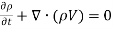( 1 )

• Conservation of impulse: the equation is shown below as Equation ( 2 ) .This equation rises from using Newton’s 2nd jurisprudence to the fluid gesture, where the rate of alteration of impulse peers the amount of the forces. The entire impulse of a system remains changeless.

( 2 )

• Conservation of energy: this equation refers to the first jurisprudence of thermodynamics, where the rate of alteration of energy of a fluid partial is equal to the rate of heat add-on plus the rate of work done. In other words, for this undertaking the energy equation histories for the heat act on the undertaking. There are many ways of showing the energy equation, one signifier is as shown in Equation 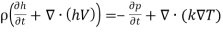( 3 )

( 3 )

3.2.2 Geometry and Boundary Conditions

Geometry:

The conventional diagram of the analysis theoretical account considered in this paper is illustrated in Figure3-2, modeled with ANSYS Fluent. The theoretical account is developed from an false physical paradigm by ignoring the structural characteristics. In order to simplify the job, the geometry of this system is specified as planar and constructed on the X, Y plane. The theoretical account geometry is scaled down to 200mm*200mm in general infinite with a thermic storage wall and two gaps as air recess and mercantile establishment ( shown in ruddy ) . All wall thicknesses are neglected in this state of affairs, which indicates the walls have zero heat conductivity opposition. There are three chief parts in this theoretical account: the air channel ( A ) , inactive solar wall ( B ) and indoor life infinite ( C ) , besides illustrated in Figure 3-2.

The thermic wall is set as 30mm*100mm. The intermediate infinite between the thermic wall and the glazing or the canal breadth is set for 20mm and the stuff to construction the thermic storage wall is H2O.

Boundary Conditionss:

The lone un-insulated surface is the interface between the thermic wall and the air channel. The other beds are insulated to either increase the thermic opposition or prevent to heat from reassigning into the internal infinite. Note that the heat flux is originally designed to move on the exterior H2O wall surface ( the surface between A and B on Figure 3-2 ) , where this surface is besides an interface between H2O and air. But mistakes occur if this interface is subjected to external heat beginning when operating in ANSYS FLUENT 15.0 bundle. Thus that in this survey, all interior wall surfaces including the roof and floor are set to be adiabatic ( under nothing heat flux ) while the thermic wall interior surface ( No. 19 on Figure 3-2 ) is capable to heat flux calculated based on the Sydney part historical informations shown in Appendix A ( Bom.gov.au, 2014 ) . However, the value of solar heat flux is non changeless during a twenty-four hours, and at this phase our cognition is non sufficient to execute a simulating based on the world parabolic behaviour of heat flux. The heat flux moving on the H2O wall for this undertaking is assumed as changeless. It is about impossible to make an accurate grading based on all fluid flow factors, to fulfill this, the H2O temperature will lift above 100EsC. To simplify the undertaking, the values are so scaled down to fulfill the theoretical account scenes by keep the same addition temperature addition rate in H2O wall. The grading computation is described below.

Initially the standard temperature for the H2O wall and theoretical account room was set the same as 300K ( 26.85EsC ) . The air temperature at recess and mercantile establishment were besides assumed changeless and tantamount to the room air temperature to simplify the undertaking. By making this, heat flux is ensured as the lone force that initiates the full system.

Other than the computational recess and mercantile establishment, the remainder of the surface boundaries are stationary walls under no-slip conditions. Resistance to flux due to friction along the surfaces is assumed negligible.

3.2.3 Imitating Parameters ( Dimensional Analysis )

From the published literature, many different parametric quantities can impact the public presentation of the H2O wall public presentation for air airing intent. As shown on Figure 3-3, there are many variables that can be investigated to optimise the H2O wall system public presentation such as wall tallness ( H ) , width ( B ) , intermediate infinite interval ( D ) and the heat flux strength moving on H2O wall surface.

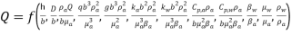
A dimensional analysis is performed to show the structural and mechanical parametric quantities that may impact the system public presentation. Buckingham theorem is the method used for dimensional analysis. First of wholly, a certain figure, “n” , of relevant dimensional physical variables are determined for this undertaking. These variables are inter-related and can be expressed via a functional relationship as shown in Equation 4, where Q stands for the mean volume flow rate at the mercantile establishment.

( 4 )

Followed by examine these parametric quantities and happen out the figure of cardinal dimensions, named “k” . Finally, by choosing “k” figure of reiterating variables, the staying ( n-k ) variables can organize ( n-k ) sets ofgroups. The elaborate working out is described in Appendix B. The solution indicates that for this undertaking analysis, there are n=16 variables, k=4 cardinal dimensions which form 12groups. Thesegroups are dimensionless groups that will impact the system public presentation. Consequently, The Buckingham Theorem consequence indicates that Q is a map of a set of dimensionless groups, which are shown below. ( 5 )

Due to constraint in clip and CFD cognition restriction at the current phase, in this survey, two factorsheat fluxstrengthandH2O wall thicknesshave been chosen as the simulating parametric quantities, therefore that the undertaking aims to analyze their effects on the system.

Solar heat flux strength is one of the most widely research parametric quantity and besides the most conclusive. Research workers find that air velocity and temperature within the solar channel of the thermal wall system increases with increasing solar heat flux strength ( Budea, 2014 )

The 2nd parametric quantity is the H2O wall thickness ( breadth ) . Presently, research workers return assorted reappraisals on the influence of H2O wall’s tallness, but besides to observe that the tallness parametric quantity is non easy to command due to realistic structural limitations. Meanwhile, there has been really limited reappraisal on the effects H2O wall thickness parametric quantity by past research workers. Comparing to the H2O wall tallness, the thickness is considered as a comparatively easy parametric quantity to command. The above grounds explain why H2O wall thickness is selected as the 2nd simulating parametric quantity to analyze for this undertaking.

3.2.4: Operating Condition

Solution Methods:

As the air flow is driven by convection in the air chamber, the system is running under force per unit area based attack. When simulating, the force per unit area field is extracted by work outing a force per unit area rectification equation which is obtained by pull stringsing the preservation of mass and impulse equations of the speed field ( Arc.vt.edu, 2014 ) . Since the government equations are non-linear, the solution procedure involves work outing the regulating equations repeatedly till the solution converges.

In this theoretical account, the perkiness consequence of air is modeled under the Boussinesq estimate. This is because the phenomenon in the solar channel is natural convection under alterations in air temperature. This estimate is used to account for the denseness fluctuation. Thus the computational theoretical account considers denseness to be changeless except for the perkiness term in the impulse equation.

Operating Parameters:

As discussed before, the two parametric quantities interested are heat flux strength and H2O wall thickness. For the heat flux strength, the scaly upper limit summer heat flux is 112; where the minimal winter 55.7. Two other heat flux strengths are chosen for comparing. The values are taken mediate the upper limit and lower limit based on tantamount increase. Therefore, the concluding four values selected for this undertaking are 55.7, 74.593.2and 112.

When analyzing the H2O wall thickness affects, the heat flux is set independent with a value of 89.2, which is the mean annual value calculated. Then the breadths selected for the H2O wall are 25mm, 30mm and 35 millimeter to compare public presentation of natural air airing of the undertaking theoretical account.

3.2.5 Convergence Criteria and Meshing

Convergence Standards

This theoretical account uses 2^neodymiumorder truth ( high declaration ) for the sing variables such as temperature and speed. All remainders are scaled and the convergence standard is said as reached when the default absolute value of the remainders are belowHowever it is of import to observe that a good initial conjecture by and large lead to a high scaled residuary and therefore the convergence standards can non be achieved. Hence after corroborating the solution conditions, a mesh independence trial is required to be performed to guarantee the solution is besides independent of the mesh. This is besides an extra critical standard to guarantee the consequences are dependable.

Finite volume method

The solution method employed in ANSYS FLUENT is known as the finite volume method under full-coupled convergent thinker. Full-coupled means that the system usually converges in less loop, but with each loop takes longer. This method operates as follows:

First of wholly, the theoretical account sphere is discretized, through the usage of mesh, into a finite set of control volumes. Next, the three regulating equations discussed before ( preservation of mass, impulse and energy ) are integrated over each single control volume to make algebraic equations for the terra incognitas. Followed by all the equations developed all being solved to give updated consequences of the dependent variables. Consequently, an approximative value of each dependant variable at any points on the sphere can be obtained.

Mesh Independency Test

A all right mesh reduces the elaboration of mistakes during the extension of the solution. However, by bettering the truth of the simulation consequences through refinement mesh, the clip devouring for computational analysis is increased correspondingly. As a consequence, a mesh independence trial was performed to guarantee the appropriate mesh is used for this system. More specifically, this means that the mesh chosen is capable of bring forthing a comparatively accurate consequence but less clip devouring. Without executing the mesh independency trial, the solutions will hold a high opportunity of changing with the polish of mesh and this clearly is non acceptable for the undertaking. The polish procedure is repeated with incrementally reduced alternations in consequence until a solution that is independent of mesh is generated.

The overall theoretical account sphere is foremost divided into 100*100 computational cells, and so traveling to 200*200, 400*400 cells for the mesh independence trial. The spheres near to interfaces were set with smaller grid spacing ( or finer mesh ) , the interior infinite set with larger grid spacing ( or courser mesh ) to better the truth. Two parametric quantities set as proctors are area-weighted mean temperature of the H2O wall and the mean volume flow rate at the mercantile establishment. There is no specific standard for the per centum difference between two back-to-back sets, but it is required to be moderately bantam to guarantee that no important effects take topographic point on the system when mesh alterations.

The differences between the sets of consequences are analyzed in per centum by sing 400*400 engagement as mention. The consequences are besides expressed in x-y chart for better ocular comparing. The elaborate informations for mesh trial including the ocular comparing figures is shown in Appendix C. A comparing of consequences is shown in Table 3-2 below.

By analyzing the consequences, it is observed that the differences between the 200*200 and 400*400 mesh are zero and less than 0.01 % for temperature and volume flow rate proctors severally. Therefore, it is believed that the 200*200 grid system has sensible imitating clip ingestion and can obtain good truth consequences for the undertaking. The mesh form is presented in Figure3-4. The observation gives the assurance that the fake solution is considered as independent of its grid.

Cite this Page

Parameters for a Computational Fluid Dynamics Analysis. (2018, Jul 22). Retrieved from https://phdessay.com/parameters-for-a-computational-fluid-dynamics-analysis/

copy to clipboard